Introduction: The Growing Need for Advanced Vehicle Diagnostics
In today’s rapidly evolving automotive landscape, the sheer volume and complexity of vehicles on the roads are increasing exponentially. Modern automobiles boast intricate internal structures, diverse models, and sophisticated systems, leading to a wide array of potential faults that can be incredibly challenging to diagnose. Many automotive maintenance enterprises find themselves struggling to keep pace, often lacking the expert technical guidance necessary to effectively repair these complex issues and meet the evolving maintenance demands of vehicle owners. To maximize vehicle uptime and minimize economic losses, drivers are increasingly seeking convenient and reliable methods for vehicle fault detection, desiring a clear understanding of their vehicle’s real-time operational status.
This is where the power of Car Diagnosis Expert Systems comes into play. Born from the field of artificial intelligence, which began its development in the 1960s, expert systems represent a pivotal application area within AI. These intelligent computer programs are designed to emulate the knowledge and reasoning of human experts, enabling them to tackle complex, domain-specific problems. Over decades of refinement, expert systems have proliferated across various professional fields, demonstrating widespread utility and continued development in practical applications. Characterized by their heuristic nature, transparency, and flexibility, these systems offer a powerful approach to problem-solving in intricate domains like automotive repair.
Understanding Car Diagnosis Expert Systems
A car diagnosis expert system is designed to mirror the diagnostic thought processes of seasoned automotive technicians, effectively identifying and resolving vehicle malfunctions. These systems primarily leverage built-in vehicle sensors to gather fault information from electronic control units (ECUs). Employing sophisticated artificial intelligence algorithms, they process this comprehensive data, analyze the root causes of failures, and deliver clear diagnostic results to users. The scope of these systems encompasses a wide range of vehicle components, including engines, chassis, and electrical systems. Fault diagnosis stands as a crucial application of artificial intelligence within the automotive industry, representing a synergistic outcome of collaboration between domain experts and software engineers.
Currently, various models of car diagnosis expert systems exist, each with its own strengths. These include rule-based systems that rely on predefined rules, instance-based systems that learn from past examples, behavior-based systems that model system behavior, fuzzy logic-based systems that handle uncertainty, and artificial neural network-based systems that mimic the human brain’s learning process. While significant progress has been made in the development of automotive fault diagnosis expert systems, they are not yet capable of fully replicating the nuanced and adaptable thinking of human experts. For optimal diagnostic outcomes, these systems often function best in collaboration with human experts in the field.
The primary limitations of current car diagnosis expert systems revolve around knowledge acquisition and the comprehensiveness of their knowledge base. The challenge of effectively acquiring and integrating expert knowledge remains a significant hurdle hindering their wider adoption and further advancement. In recent years, researchers have been actively exploring innovative approaches to overcome these limitations and enhance the capabilities of expert systems. The future evolution of car diagnosis expert systems is anticipated to be driven by advancements in networking, intelligence, and seamless integration within broader automotive systems.
The Rise of Neural Network-Based Car Diagnosis Expert Systems
The development of intelligent car diagnosis expert systems is not just a trend; it’s an inevitable necessity driven by the rapid advancements in the automotive industry. A particularly promising direction in recent years has been the integration of neural network technology into these systems. This integration marks a significant leap forward in automotive research and technology. From both theoretical and practical standpoints, neural network-based fault diagnosis systems offer distinct advantages in areas such as knowledge acquisition, knowledge representation, reasoning, learning capacity, and fault tolerance.
Building upon the inherent characteristics of expert systems, this discussion will delve into the design and implementation of a car diagnosis expert system specifically leveraging neural network technology. The objective is to showcase how intelligent fault diagnosis can be effectively realized, providing valuable tools for identifying and rectifying vehicle faults, and demonstrating the practical significance of these systems in the automotive domain.
Fig. 2: System structure of a feed forward neural network with three layers, illustrating the flow of information from input to output through hidden layers.
BP Neural Networks: A Foundation for Intelligent Diagnosis
Neural networks are fundamentally information processing systems or computational models inspired by the structure and functionality of the human brain. These networks are renowned for their robust learning and memorization capabilities, coupled with sophisticated intelligent processing, making them invaluable across diverse fields including automatic control, artificial intelligence, pattern recognition, and, crucially, fault diagnosis.
Structure and Function of Neural Networks
The neuron, the basic building block of a neural network, can be visualized as a multi-input, single-output nonlinear processing unit. Its internal state is determined by the weighted sum of its input signals. A neural network is composed of numerous interconnected neurons organized in layers. Based on their connection configurations and functional roles, neural networks are broadly categorized into two primary types: feedforward networks and feedback networks.
Feedforward Neural Networks
Feedforward networks represent the most prevalent type of neural network architecture. As depicted in Fig. 2, in a feedforward network, neurons are organized in layers, and information flows unidirectionally from the input layer, through one or more hidden layers, to the output layer. Each neuron receives inputs from the preceding layer and transmits its output to the subsequent layer. Notably, feedforward networks lack feedback loops, meaning there are no connections that loop back to previous layers.
The network nodes are classified as either input units or computational units. Each computational unit can receive multiple inputs but produces only a single output. Feedforward networks are typically structured in distinct layers. Input and output nodes serve as interfaces with the external environment, while intermediate layers are designated as hidden layers. This layered structure forms a powerful learning system that is both conceptually straightforward and relatively easy to program. From a systems perspective, feedforward networks embody static nonlinear mapping. While most feedforward neural networks do not explicitly model dynamic system behavior, they excel in tasks such as classification and pattern recognition, often surpassing other neural network types in these capabilities.
Feedback Neural Networks
Feedback neural networks, also known as recurrent or regression networks, introduce feedback connections, allowing signals to travel in loops. In these networks, the input signal sets the initial state of the system. Through a series of state transitions, the network gradually converges toward an equilibrium state. Consequently, the stability of feedback networks is a critical consideration. In contrast to feedforward networks, all nodes in a feedback neural network function as computational units, capable of both receiving inputs and producing outputs to the external environment and to other neurons within the network.
BP Neural Networks: Backpropagation for Learning
Artificial neural networks, particularly the Backpropagation (BP) neural network, have found extensive applications in pattern recognition and related domains. The BP neural network, a multilayer feedforward network, is particularly well-suited for fault diagnosis applications. Typically, neurons in BP networks employ a sigmoid activation function, known for its differentiability. The learning process in a BP network involves the backpropagation algorithm, a supervised learning technique. This algorithm minimizes the error between the network’s actual output and the desired output by iteratively adjusting the connection weights between neurons. During training, error signals propagate backward through the network, guiding the weight adjustments to reduce the overall error. This iterative process allows the network to learn complex patterns and relationships from training data.
Calculation and Learning in BP Neural Networks
Consider the neural network architecture illustrated in Fig. 2, assuming it has M input nodes and L output nodes, with a single hidden layer containing q neurons. During the training phase, with N training samples, let’s denote the input and desired output of the p-th sample as Xp and dp, respectively. The input (in_i) and output (O_i) of the i-th neuron in the hidden layer under the influence of the p-th sample can be expressed mathematically as:
Equation 1: in_i = ∑(w_ij * x_j) (summation over j from 1 to M)
Equation 2: O_i = f(in_i)
Where:
- w_ij represents the connection weight between the j-th input node and the i-th hidden neuron.
- x_j is the j-th input component of the sample p.
- f(.) is the Sigmoid activation function, introducing non-linearity.
The derivative of the Sigmoid output function, crucial for backpropagation, is given by:
Equation 3: f'(in_i) = O_i * (1 – O_i)
The output O_i from the hidden layer neurons is then transmitted forward to the k-th neuron in the output layer, serving as one of its inputs. The input (in_k) and output (y_k) of the k-th neuron in the output layer are calculated as:
Equation 4: in_k = ∑(v_ki * O_i) (summation over i from 1 to q)
Equation 5: y_k = f(in_k)
Where:
- v_ki represents the connection weight between the i-th hidden neuron and the k-th output neuron.
- O_i is the output of the i-th hidden neuron.
If the network output y_k deviates from the desired output d_k for a given sample pair, an error signal is propagated backward through the network. During this backpropagation process, the connection weights (w_ij and v_ki) are iteratively adjusted to minimize the error until the output layer neurons produce the desired output values. This weight adjustment is guided by optimization algorithms, such as gradient descent, to effectively learn from the training data. After adjusting weights for sample p, the process is repeated for subsequent samples until all N training samples have been processed.
Adjusting Network Weighted Coefficients
For each training sample p, a quadratic error function (J_p) is introduced to quantify the discrepancy between the desired output and the actual network output:
Equation 6: J_p = 0.5 * ∑(d_k – y_k)^2 (summation over k from 1 to L)
The total error function (J) across all N training samples is then the sum of individual sample errors:
Equation 7: J = ∑(J_p) (summation over p from 1 to N)
The objective of the training process is to minimize this total error function J. This is achieved by iteratively modifying the connection weights in the direction that reduces J.
The correction formulas for the weights connecting the input layer to the hidden layer (Δw_ij) and the hidden layer to the output layer (Δv_ki) are derived using gradient descent and backpropagation principles:
Equation 8: Δv_ki = η (d_k – y_k) f'(in_k) * O_i
Equation 9: Δw_ij = η ∑((d_k – y_k) f'(in_k) v_ki f'(in_i) * x_j) (summation over k from 1 to L)
Where:
- η is the learning rate, a parameter controlling the step size of weight adjustments (typically a small positive value, 0 < η < 1).
To enhance the learning process and prevent oscillations, an inertia term (momentum) is often incorporated. The weight correction formulas with momentum become:
Equation 10: Δv_ki(t+1) = η (d_k – y_k) f'(in_k) O_i + α Δv_ki(t)
Equation 11: Δw_ij(t+1) = η ∑((d_k – y_k) f'(in_k) v_ki f'(in_i) x_j) + α Δw_ij(t)
Where:
- α is the inertia coefficient (momentum), typically in the range 0 < α < 1, influencing the contribution of previous weight changes to the current update.
- t and t+1 represent iteration steps.
Summary of the BP Neural Network Learning Process:
- Initialization: All connection weights are initialized to small random values.
- Sample Presentation: A training sample (input vector X_n and desired output vector d_n) is presented to the network.
- Error Calculation: The error between the network’s actual output and the desired output is computed.
- Output Layer Weight Adjustment: The weight adjustments for connections leading to the output layer are calculated and applied.
- Hidden Layer Weight Adjustment: The weight adjustments for connections leading to the hidden layer are calculated and applied using backpropagation.
- Iteration: Steps 3-5 are repeated for all training samples iteratively until the error reaches a predefined acceptable level or a maximum number of iterations is reached.
Fault Diagnosis Expert System Based on Neural Networks: Combining Strengths
Traditional expert systems rely heavily on logical reasoning, progressing through stages of knowledge acquisition, representation, and inference. This process can be time-consuming and knowledge acquisition can be a bottleneck. In contrast, neural networks mimic the human brain’s approach to artificial intelligence, learning from vast amounts of data and events. Expert systems and artificial neural networks represent complementary approaches to problem-solving. Combining these methodologies allows for leveraging their unique strengths, creating more robust and practical AI applications capable of tackling complex problems that neither approach could solve effectively in isolation.
Structure and Knowledge Flow in Neural Network Expert Systems
The fundamental architecture of a neural network-based expert system is depicted in Fig. 1. This architecture facilitates automatic input acquisition, organization, and storage of learning examples provided by domain experts.
The process begins with selecting an appropriate neural network architecture and invoking a suitable learning algorithm. This enables the system to acquire knowledge, which is then encoded within the network’s connection weights, forming the knowledge base. When new learning instances are introduced, the knowledge acquisition module automatically updates the network weights, refining the knowledge base based on the new information.
Knowledge Acquisition, Representation, and Inference
Knowledge Acquisition: In a neural network, knowledge acquisition is achieved by training the network to produce outputs that closely align with expert-provided answers for given inputs. The goal is to imbue the network with problem-solving capabilities comparable to those of domain experts. This knowledge acquisition process is analogous to how biological neural networks adapt, with intelligent behavior emerging from adjustments in the connection strengths between neurons.
Knowledge Representation: Knowledge can be formalized as specific examples, which neural networks can readily learn from. The process involves:
- Defining the neural network model and topology.
- Selecting a suitable learning algorithm.
- Training the network using example data.
During training, the network adjusts its weights, effectively storing the acquired knowledge. Multilayer feedforward neural networks trained with supervised learning are a common and effective approach. After normalizing the data, numerical sample sets are constructed. In the learning phase, network weights are adjusted based on the error between the network’s output and the desired output. The network training continues until the error is minimized to an acceptable level. At this point, the neural network has effectively learned from the provided examples and stored this knowledge within its structure.
Inference Mechanism: Neural networks offer efficient inference capabilities. The inference mechanism in a fault diagnosis expert system can employ direct reasoning, backward reasoning, or a hybrid approach. Neural network-based systems typically utilize direct reasoning. The trained network performs computations, starting from an initial state and progressing forward until a target state (diagnosis) is reached. This reasoning process is essentially a forward calculation. By inputting a known symptom vector, the network calculates the output, providing a fault vector indicative of the likely fault.
Compared to traditional expert systems, this direct reasoning approach in neural network expert systems offers several advantages, including rapid inference and inherent conflict resolution.
Designing an Automobile Fault Diagnosis Expert System with Neural Networks
A neural network-based fault diagnosis expert system can effectively identify fault types by training the network with diverse sets of fault examples. Once trained, the system can swiftly analyze new input information and accurately determine the type of failure present in the equipment or system under diagnosis.
Case Study: Engine Abnormal Sound Analysis
Vehicle condition deteriorates over time and mileage, often manifested through symptoms like abnormal sounds, fluid leaks, overheating, power loss, excessive fuel consumption, and vibrations.
Table 1: Codes and Fault Phenomena of Abnormal Engine Sounds
| Code | Fault Phenomenon | Code | Fault Phenomenon |
|---|---|---|---|
| x1 | Engine knock during cold start | x10 | Noise from exhaust manifold or pipe |
| x2 | Engine knock when accelerating | x11 | Noise from air filter |
| x3 | Engine knock when decelerating | x12 | Abnormal noise from generator |
| x4 | Irregular engine knock | x13 | Abnormal noise from power steering pump |
| x5 | Engine knock when idling | x14 | Abnormal noise from air conditioner compressor |
| x6 | Metallic knock | x15 | Noise from valve mechanism |
| x7 | Deep engine knock | x16 | Noise from cylinder head |
| x8 | Crisp engine knock | x17 | Noise from timing belt or chain |
| x9 | Noise from intake manifold |
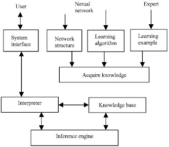
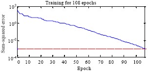
Table 1: A compilation of fault phenomena associated with abnormal engine sounds, categorized by codes x1 to x17.
Failures in automotive mechanical systems frequently manifest as abnormal noises. The engine, a complex assembly, can generate noise for numerous reasons. Abnormal engine sounds serve as valuable indicators of potential faults, carrying rich diagnostic information.
This study focuses on designing a car diagnosis expert system based on neural networks, using abnormal engine sounds as a practical example. Engine noise arises from vibrations or sound waves emanating from engine components. The presence of abnormal sounds often signals underlying engine faults. Common abnormal engine sounds include piston cylinder knocking, piston pin knocking, connecting rod bearing knocking, and crankshaft bearing knocking. These are categorized with codes y1, y2, y3, and y4, respectively, and are associated with the 17 fault phenomena listed in Table 1.
Neural Network Architecture for Fault Diagnosis
The structure of the neural network is determined by the number of fault phenomena and the types of faults to be diagnosed. Based on the analysis, a three-layer BP neural network is selected. The input layer has 17 nodes, corresponding to the 17 fault phenomena of abnormal engine sounds. The output layer has 4 nodes, representing the four types of abnormal engine sounds (y1-y4).
Determining the optimal number of hidden layer nodes is more intricate. Too few nodes may limit the network’s learning capacity and fault tolerance, while too many nodes can lead to prolonged training times and may not necessarily improve accuracy. An empirically derived formula provides guidance for estimating the number of hidden layer nodes (n2):
Equation 12: n2 = √(n1 + n3) + α
Where:
- n1 is the number of input layer nodes (17).
- n3 is the number of output layer nodes (4).
- α is an adjustable value in the range [1, 10].
Considering these factors, and through experimentation, the number of hidden layer nodes (n2) is set to 7 for this expert system.
Sample Selection and Training:
Based on fault diagnosis scenarios, training samples and desired outputs are defined, as shown in Tables 2 and 3.
Table 2: Training Samples – Fault Phenomena of Abnormal Engine Sounds
| Sample | x1 | x2 | x3 | x4 | x5 | x6 | x7 | x8 | x9 | x10 | x11 | x12 | x13 | x14 | x15 | x16 | x17 |
|---|---|---|---|---|---|---|---|---|---|---|---|---|---|---|---|---|---|
| 1 | 1 | 1 | 0 | 1 | 0 | 1 | 0 | 1 | 0 | 0 | 0 | 0 | 0 | 0 | 1 | 0 | 0 |
| 2 | 0 | 1 | 1 | 0 | 1 | 0 | 1 | 0 | 1 | 0 | 0 | 0 | 1 | 0 | 0 | 1 | 0 |
| 3 | 1 | 0 | 1 | 1 | 0 | 0 | 0 | 1 | 0 | 1 | 0 | 1 | 0 | 0 | 0 | 0 | 1 |
| 4 | 0 | 0 | 0 | 0 | 1 | 1 | 1 | 0 | 0 | 0 | 1 | 0 | 0 | 1 | 1 | 1 | 0 |
| 5 | 1 | 1 | 1 | 0 | 0 | 1 | 0 | 0 | 1 | 1 | 0 | 0 | 0 | 0 | 0 | 0 | 0 |
| 6 | 0 | 1 | 0 | 1 | 1 | 0 | 1 | 1 | 0 | 0 | 1 | 0 | 0 | 0 | 1 | 0 | 1 |
| 7 | 1 | 0 | 0 | 0 | 0 | 1 | 1 | 1 | 1 | 0 | 0 | 1 | 1 | 0 | 0 | 1 | 0 |
| 8 | 0 | 0 | 1 | 1 | 1 | 0 | 0 | 0 | 0 | 1 | 1 | 0 | 0 | 1 | 1 | 0 | 1 |
Table 2: Eight training samples representing different combinations of fault phenomena (x1-x17) associated with abnormal engine sounds.
Table 3: Desired Outputs – Abnormal Engine Sounds
| Sample | y1 | y2 | y3 | y4 |
|---|---|---|---|---|
| 1 | 1 | 0 | 0 | 0 |
| 2 | 0 | 1 | 0 | 0 |
| 3 | 0 | 0 | 1 | 0 |
| 4 | 0 | 0 | 0 | 1 |
| 5 | 1 | 0 | 0 | 0 |
| 6 | 0 | 1 | 0 | 0 |
| 7 | 0 | 0 | 1 | 0 |
| 8 | 0 | 0 | 0 | 1 |
Table 3: Desired output codes (y1-y4) corresponding to the abnormal engine sounds for each training sample.
Training Results and Analysis:
In this car diagnosis expert system based on a BP neural network, the training error is set to 0.001. The training samples are input into the system, and the test results are presented in Table 4.
Table 4: Actual Network Output After Training
| Sample | y1 | y2 | y3 | y4 |
|---|---|---|---|---|
| 1 | 0.9988 | 0.0012 | 0.0013 | 0.0014 |
| 2 | 0.0015 | 0.9985 | 0.0011 | 0.0012 |
| 3 | 0.0012 | 0.0014 | 0.9987 | 0.0011 |
| 4 | 0.0011 | 0.0013 | 0.0012 | 0.9989 |
| 5 | 0.9989 | 0.0011 | 0.0012 | 0.0013 |
| 6 | 0.0013 | 0.9987 | 0.0014 | 0.0011 |
| 7 | 0.0014 | 0.0012 | 0.9988 | 0.0013 |
| 8 | 0.0012 | 0.0011 | 0.0013 | 0.9988 |
Table 4: Actual output values from the BP neural network after training, demonstrating close approximation to the desired outputs.
As evident from Tables 3 and 4, the actual network outputs closely match the desired output values, indicating a high degree of accuracy and reliability for this BP neural network-based car fault diagnosis method.
Fig. 3 illustrates the learning curve, depicting the relationship between learning error and training epochs. The graph shows that the error accuracy meets the fault diagnosis requirement after approximately 108 training steps. Furthermore, changes in the desired error level directly influence the training time and number of steps. A smaller desired error necessitates longer training time and more training steps. These results highlight the network’s robust diagnostic capabilities, provided with sufficient training data.
Conclusion: Embracing the Expertise of AI in Car Diagnostics
Car diagnosis expert systems, particularly those leveraging neural network technology, are transforming automotive repair. They offer a powerful approach to tackling the increasing complexity of modern vehicles, providing technicians and vehicle owners with efficient and accurate fault detection and diagnostic capabilities. As AI continues to advance, these systems will become even more integral to the automotive industry, driving improvements in vehicle maintenance, reducing downtime, and enhancing the overall ownership experience. The future of automotive diagnostics is undoubtedly intertwined with the ongoing evolution and refinement of car diagnosis expert systems, bringing expert-level diagnostic capabilities to a wider audience.