The automotive industry is experiencing unprecedented growth and complexity. Modern vehicles are intricate systems with diverse models and sophisticated internal structures, leading to a wide array of potential faults that can be challenging to diagnose. Many auto repair shops struggle to keep pace with these advancements, often lacking the specialized knowledge required for effective and timely repairs. This expertise gap results in prolonged vehicle downtime and increased costs for vehicle owners, highlighting the urgent need for more efficient and accessible diagnostic solutions. Car owners are increasingly seeking reliable and convenient methods to quickly identify vehicle problems and understand the real-time health of their cars.
Expert systems, a cornerstone of artificial intelligence, emerged in the 1960s and offer a promising approach to address these challenges. An expert system is essentially an intelligent computer program designed to mimic the problem-solving abilities of human experts in a specific field. By leveraging vast knowledge bases and sophisticated reasoning mechanisms, these systems can tackle complex issues that typically require expert intervention. Over decades of development, expert systems have permeated numerous professional domains, proving their versatility and effectiveness in various applications. They are characterized by their heuristic nature, transparency in reasoning, and adaptability to new information.
In the context of automotive repair, expert systems for car engine fault diagnosis can replicate the diagnostic thought processes of experienced mechanics to pinpoint and resolve vehicle malfunctions. These systems primarily utilize data from onboard sensors and electronic control units (ECUs) to gather real-time fault information. By employing artificial intelligence algorithms, they process this comprehensive data, analyze potential causes, and provide users with clear diagnostic results. The scope of these systems extends to various vehicle components, including engines, chassis, and electrical systems. Fault diagnosis is a critical application area for artificial intelligence within the automotive sector, representing a synergy between domain expertise and technological innovation.
Currently, several models of expert systems are employed for automotive fault diagnosis, including rule-based, instance-based, behavior-based, fuzzy logic-based, and artificial neural network-based systems. While significant progress has been made in this field, expert systems are not yet capable of fully replacing human expertise. Optimal diagnostic outcomes often require a collaborative approach, combining the strengths of expert systems with the nuanced judgment of human diagnosticians.
The primary limitations of current automotive fault diagnosis expert systems lie in their knowledge acquisition capabilities and the breadth of their knowledge bases. Knowledge acquisition, in particular, is a major bottleneck hindering their widespread adoption and effectiveness. Recent research efforts are exploring innovative methods to overcome these limitations and enhance the capabilities of expert systems. The future trajectory of automotive fault diagnosis expert systems points towards increased networking, enhanced intelligence, and seamless integration with other vehicle systems and diagnostic tools.
The development of intelligent fault diagnosis expert systems is not merely a technological advancement; it’s an essential evolution driven by the rapid expansion of the automotive industry. Integrating neural network technology into these systems represents a significant leap forward. Neural networks offer unique advantages in knowledge acquisition, representation, reasoning, learning, and fault tolerance. From both theoretical and practical standpoints, neural network-based fault diagnosis systems hold substantial promise for revolutionizing automotive repair.
This discussion will delve into the design and implementation of a neural network-based expert system for car engine fault diagnosis. This system aims to provide a practical tool for identifying and resolving vehicle engine issues, demonstrating the real-world value of this technology in enhancing automotive maintenance and repair.
Understanding BP Neural Networks
Neural networks are computational systems inspired by the biological structure and function of the human brain. These systems excel at learning, memorization, and complex information processing, making them invaluable across diverse fields like automatic control, artificial intelligence, pattern recognition, and fault diagnosis.
Structure of Neural Networks
The fundamental building block of a neural network is the neuron. Imagine it as a single-input, single-output non-linear processing unit. Its internal state is determined by the weighted sum of multiple input signals. A neural network is composed of numerous interconnected neurons arranged in layers. Based on their connection patterns, neural networks can be broadly categorized into two types: feedforward and feedback networks.
Feedforward Neural Networks
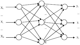
Feedforward networks are the most common type, characterized by a unidirectional flow of information. As illustrated in Fig. 1, neurons in each layer receive input from the preceding layer and transmit their output to the subsequent layer. There are no feedback loops within the network.
Fig. 1: System structure of a three-layer feedforward neural network.
Within a feedforward network, nodes are classified as either input units or processing units. Each processing unit can accept multiple inputs but produces only a single output. Feedforward networks are typically structured in layers. The input and output layers interface with the external environment, while intermediate layers are known as hidden layers. This layered architecture creates a powerful learning system that is structurally simple and relatively easy to program. From a systems perspective, feedforward networks represent static non-linear mappings. While they may not focus on dynamic system behavior, they are particularly strong in classification and pattern recognition tasks compared to other neural network types.
Feedback Neural Networks
Feedback neural networks, also known as recurrent or regression networks, incorporate feedback loops. In these networks, the input signal sets the initial state, and the system evolves through a series of state transitions until it reaches a stable equilibrium. Stability is a critical consideration in feedback networks. All nodes in a feedback network act as processing units, capable of both receiving inputs and generating outputs.
BP Neural Networks
Among the various types of artificial neural networks used in pattern recognition and other applications, Backpropagation (BP) neural networks are particularly prevalent. BP networks are multilayer feedforward networks well-suited for fault diagnosis. Typically, neurons in BP networks employ a Sigmoid activation function. The network’s learning process involves a least mean squares algorithm. During training, the error between the network’s actual output and the desired output propagates backward through the network. This backpropagation of error adjusts the connection weights between neurons to minimize the mean squared error.
Calculation in Feedforward Neural Networks
Consider the feedforward neural network in Fig. 1, assuming M input nodes and L output nodes with a single hidden layer containing q neurons. During the network training phase, N training samples are used. For sample p, input Xp and desired output dp are used to train the network. The input and output of neuron i in the hidden layer are calculated as follows:
Equation 1: $Inputi^p = sum{j=1}^{M} w_{ij} x_j^p$
Equation 2: $O_i^p = f(Input_i^p)$
Where:
- $w_{ij}$ is the weight of the connection between input node j and hidden neuron i.
- $x_j^p$ is the j-th input of sample p.
- $O_i^p$ is the output of hidden neuron i for sample p.
- $f(.)$ is the Sigmoid activation function.
The derivative of the Sigmoid activation function is given by:
Equation 3: $f'(x) = f(x)(1-f(x))$
The output $O_i^p$ from the hidden layer is then transmitted forward to neuron k in the output layer, serving as one of its inputs. The input and output of neuron k in the output layer are calculated as:
Equation 4: $Inputk^p = sum{i=1}^{q} v_{ik} O_i^p$
Equation 5: $y_k^p = f(Input_k^p)$
Where:
- $v_{ik}$ is the weight of the connection between hidden neuron i and output neuron k.
- $y_k^p$ is the output of output neuron k for sample p.
If the output $y_k^p$ deviates from the desired output $d_k^p$, an error signal is propagated backward through the network. During this backpropagation, the connection weights are iteratively adjusted until the output layer neurons produce the desired output values. After adjusting the weights based on sample p, the process is repeated for the next sample until all N training samples have been processed.
Adjustment of Network Weights
For each sample p, a quadratic error function is introduced:
Equation 6: $Ep = frac{1}{2} sum{k=1}^{L} (d_k^p – y_k^p)^2$
The total error function across all N training samples is:
Equation 7: $J = sum_{p=1}^{N} E_p$
The network aims to minimize the error function J by adjusting the weights in the direction of decreasing $J_p$.
The weight correction formulas for connections to the hidden and output layers are:
Equation 8: $Delta v_{ik} = -eta frac{partial Ep}{partial v{ik}} = eta delta_k^p O_i^p$
Equation 9: $Delta w_{ij} = -eta frac{partial Ep}{partial w{ij}} = eta gamma_i^p x_j^p$
Where $eta$ is the learning rate (0 < $eta$ < 1).
The weight correction formulas for arbitrary neurons k (output layer) and i (hidden layer) under sample p are:
Equation 10: $v{ik}(t+1) = v{ik}(t) + Delta v{ik} + alpha (v{ik}(t) – v_{ik}(t-1))$
Equation 11: $w{ij}(t+1) = w{ij}(t) + Delta w{ij} + alpha (w{ij}(t) – w_{ij}(t-1))$
Where $alpha$ is the momentum coefficient (0 ≤ $alpha$ < 1).
The iterative learning process for weight adjustment is summarized below:
- Initialize all weights to small random values.
- Present the training set with input vectors $X_n$ and desired output vectors $d_n$.
- Calculate the error between the network’s actual output and the desired output.
- Compute and adjust the weights for the output layer connections.
- Compute and adjust the weights for the hidden layer connections.
- Repeat steps 3-5 until the error meets the system’s requirements.
Fault Diagnosis Expert Systems Powered by Neural Networks
Traditional expert systems rely on logical reasoning through stages like knowledge acquisition, representation, and inference, which can be time-consuming. Neural networks, on the other hand, mimic the human brain’s ability to learn from vast amounts of data and respond to events. Expert systems and neural networks offer complementary strengths. Combining them can create powerful and practical AI systems capable of tackling complex problems that neither approach can solve effectively alone.
Structure of Neural Network Expert Systems
The basic architecture of a neural network expert system is shown in Fig. 2. It can automatically process input data and learn from expert-provided examples.
Fig. 2: Basic structure of a neural network expert system.
By selecting an appropriate neural network architecture and learning algorithm, the system can acquire knowledge for its knowledge base. When new data is introduced, the knowledge acquisition module updates the network weights, effectively refining the knowledge base through continuous learning.
Knowledge Acquisition with Neural Networks
Knowledge acquisition in neural networks involves training the system to produce outputs that closely match expert opinions under similar input conditions. This aims to equip the network with problem-solving capabilities comparable to domain experts. Neural networks, inspired by biological systems, represent knowledge through the patterns of connections and weights between artificial neurons.
Knowledge can be formalized as specific examples, which neural networks can readily learn from. The process begins by defining the network model and topology, followed by training using a chosen learning algorithm. Through training, the network adjusts its weights, effectively acquiring and storing knowledge. Multilayer feedforward networks with supervised training are commonly used. After data normalization, numerical sample sets are created. During training, network weights are adjusted based on the error between the network’s output and the desired output. The training continues until the mean squared error falls below a predefined threshold, at which point the network has effectively learned from the provided examples and encoded this knowledge in its structure.
Knowledge Representation in Neural Networks
Neural networks represent knowledge in primarily two ways:
-
Rule-based Representation: Expert knowledge is translated into production rules (IF-THEN rules) and stored in the knowledge base. These rules represent expert experience in a structured, logical format.
-
Data-driven Learning: Neural networks are trained on historical data or expert experiences to discover new diagnostic rules and expand the knowledge base. This self-learning capability is a key advantage of neural network-based expert systems for fault diagnosis, enabling them to adapt and improve over time.
Inference Mechanism in Neural Networks
Fault diagnosis expert systems employ various inference mechanisms, including forward reasoning, backward reasoning, and mixed reasoning. Neural network-based systems typically use forward reasoning (also known as direct reasoning). The trained neural network performs computations, starting from an initial state and progressing forward until a target state (diagnosis) is reached. This reasoning method is essentially the forward calculation process within the network. The system takes known symptoms as input, processes them through the network, and outputs a fault vector representing the diagnosis.
Compared to traditional expert systems, this direct reasoning approach in neural network-based systems offers advantages such as faster inference speeds and the ability to handle conflicting information more effectively.
Designing a Neural Network-Based Automobile Fault Diagnosis Expert System
A neural network-based fault diagnosis expert system can identify the type of fault in a device once it has been trained on a diverse set of fault examples. After training, the network can quickly analyze new input data and determine the nature of any equipment malfunction.
Failure Mode Analysis of Engine Abnormal Sounds
Over time and with increasing mileage, vehicle condition inevitably deteriorates. This is often signaled by symptoms like abnormal noises, fluid leaks, overheating, power loss, excessive fuel consumption, and vibrations.
Table 1: Codes and fault phenomena of abnormal automobile engine sounds.
Table 1 lists fault phenomena (xi) associated with abnormal engine sounds.
Mechanical system failures in vehicles are frequently indicated by unusual noises. The engine, being a complex assembly, can produce noises for various reasons. Abnormal engine sounds are often a crucial indicator of underlying problems, carrying valuable diagnostic information.
This study designs a neural network-based fault diagnosis expert system using abnormal engine sounds as a case study. Engine noise originates from vibrations and sound waves produced by engine components. Abnormal sounds suggest potential faults. Common abnormal engine sounds include piston cylinder knocking, piston pin knocking, connecting rod bearing knocking, and crankshaft bearing knocking. These are categorized as codes y1, y2, y3, and y4, respectively, and are associated with 17 fault phenomena as detailed in Table 1.
Establishing the Fault Diagnosis Neural Network
The size of the neural network is determined by the number of abnormal sound symptoms and the types of faults to be diagnosed. Based on the analysis, a three-layer BP neural network is chosen, featuring 17 input nodes (corresponding to the 17 fault phenomena) and 4 output nodes (representing the four types of abnormal engine sounds).
Determining the optimal number of hidden layer nodes is more complex. Too few nodes may hinder network training and pattern recognition, leading to poor fault tolerance. Conversely, too many nodes can prolong training time without necessarily improving accuracy. An optimal number of hidden layer nodes exists. An empirical formula guides the selection of the hidden layer node count:
Equation 12: $n_2 = sqrt{n_1 + n_3} + alpha$
Where:
- $n_1$ is the number of input layer nodes (17).
- $n_3$ is the number of output layer nodes (4).
- $alpha$ is an adjustment value in the range [1, 10].
Considering these factors, the number of hidden layer nodes ($n_2$) is set to 7 for this expert system.
Sample Selection for Neural Network Training
Based on fault diagnosis scenarios, training samples and corresponding outputs are prepared, as shown in Table 2 and Table 3.
Table 2: Eight training samples of fault phenomena for abnormal engine sounds in the BP neural network expert system.
Table 2 lists input training samples (xi) representing fault phenomena.
Table 3: Eight output samples of abnormal engine sounds for the BP neural network expert system.
Table 3 lists desired output samples (yi) representing abnormal engine sounds.
Table 4: Actual output of the BP neural network when training samples are input.
Table 4 shows the actual network outputs (yi) after training.
Training Results and Analysis
In this BP neural network-based automobile fault diagnosis expert system, the training error target is set to 0.001. After inputting the training samples into the system, the test results are obtained, as shown in Table 4.
Comparing Table 3 and Table 4, the actual outputs closely match the desired outputs, indicating the high accuracy and reliability of this BP neural network-based fault diagnosis method.
Fig. 3: Learning error vs. training epochs.
Fig. 3 illustrates the relationship between learning error and training epochs. The graph shows that the error target is achieved after 108 training epochs, meeting the fault diagnosis requirements. Furthermore, modifying the error requirement reveals a corresponding change in training time and epochs. Lower error targets necessitate longer training times and more epochs. The results demonstrate the network’s robust diagnostic capabilities when provided with sufficient training data.